Thematic maps
The R Script associated with this page is available here. Download this file and open it (or copy-paste into a new script) with RStudio if you want to follow along.
1 Visualizing spatial data
In previous exercises we have already used plotting functionalities through the plot() command. Here we will highlight a few other ways for visualizing spatial data.
The most comprehensive way of creating visualizations is using the ggplot2 package, which in newer version also supports rendering sf objects directly.
Unfortunately this tutorial won’t be able go into details of all functionalities of the ggplot2 package. There are however several free tutorials online. Also see Resources.
suppressPackageStartupMessages(library(ggplot2))
library(sf)
## Linking to GEOS 3.8.0, GDAL 3.0.4, PROJ 6.3.1library(dplyr)## Warning: package 'dplyr' was built under R version 4.0.3##
## Attaching package: 'dplyr'## The following objects are masked from 'package:stats':
##
## filter, lag## The following objects are masked from 'package:base':
##
## intersect, setdiff, setequal, union# Load a shapefile of the world from the tmap package
# (in sf format)
data('World',package = 'tmap')
# Which five countries have the lowest human footprint
lhfp <- World %>% dplyr::arrange(footprint) %>% dplyr::slice(1:5)
# Create the plot
ggplot(World) +
theme_minimal() +
geom_sf(aes(fill = log10(pop_est))) +
scale_fill_viridis_b() +
# Insert labels for countries with low hfp
geom_sf_label(data = lhfp, aes(label = name))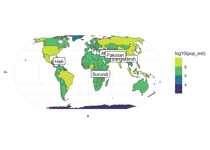
Creating good looking ggplot figures can take quite some time and constant practise is recommended.
Have a look at the colorspace package for creating some good colour ramps for figures that are colorblind friendly and offer decent contrast. See colorspace::choose_palette() and colorspace::hcl_palettes()
1.1 Thematic mapping with tmap
The tmap package has been specifically created for creating thematic maps that are visually pleasing. In my opinion advantage of using tmap over ggplot is that styles and legends are generally easier to add to a figure, making the production workflow less of an effort.
library(tmap)
library(sf)

data("World",package = 'tmap')
data('land',package = 'tmap')

# mapping maximum hail sizes
mapw <- tm_shape(World) +
  tm_graticules() +
  tm_polygons(col = 'life_exp', title = "Life expectancy", lwd = 1.2) +
  tm_text("iso_a3", size = "AREA", col = "grey30", root = 3) +
  tm_legend(title = "",
            legend.position = c("left", "bottom"), scale=1.2) +
  tm_layout(frame = FALSE,
            title.position = c("left", "top"),
            inner.margins = c(0.10, 0, 0.08, 0)) +
  tm_credits("Here could be some descriptive text or credits.", align="left", position = c(0.2, 0), size = 0.6)

mapw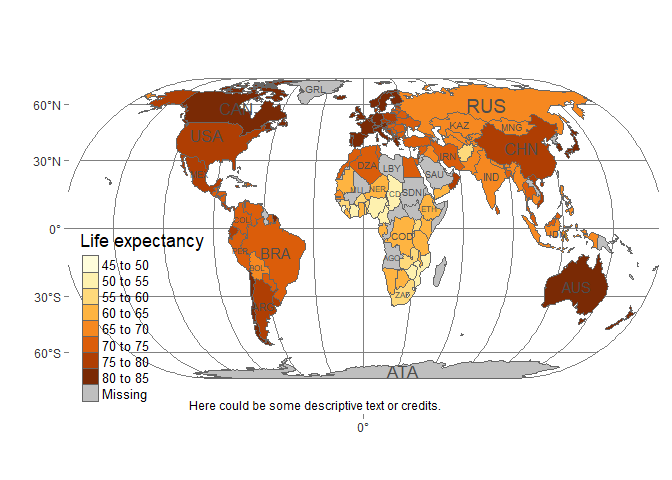
# It is also possible to save this map
#tmap_save(mapw, "lifexp.png", dpi=300)
Looks pretty easy for the little bit of code, right? More information can be found on the CRAN vignette. Really nice examples of tmap created maps (including code) can also be found on the github page.
1.2 The cartography package
Another package that can create very pretty thematic maps, is the cartography package which has evolved besides the tmap package. However in contrast to ´tmap´ the cartography package provides overlay functions that supplement default sf plots. To be honest, I haven’t used it before and thus will - in the interest of time - only show the examples from the vignette.
library(sf)
library(cartography)
## Warning: package 'cartography' was built under R version 4.0.3# import to an sf object
mtq <- st_read(dsn = system.file("gpkg/mtq.gpkg", package="cartography"), quiet = TRUE)
# Plot the municipalities
plot(st_geometry(mtq), col="darkseagreen3", border="darkseagreen4",
bg = "lightblue1", lwd = 0.5)
# Plot symbols with choropleth coloration
propSymbolsChoroLayer(
x = mtq,
var = "POP",
border = "grey50",
lwd = 1,
legend.var.pos = "topright",
legend.var.title.txt = "Population",
var2 = "MED",
method = "equal",
nclass = 4,
col = carto.pal(pal1 = "sand.pal", n1 = 4),
legend.var2.values.rnd = -2,
legend.var2.pos = "left",
legend.var2.title.txt = "Median\nIncome\n(in euros)"
)
# layout
layoutLayer(title="Population & Wealth in Martinique, 2015",
author = "cartography 2.1.3",
sources = "Sources: Insee and IGN, 2018",
scale = 5, tabtitle = TRUE, frame = FALSE)
# north arrow
north(pos = "topleft")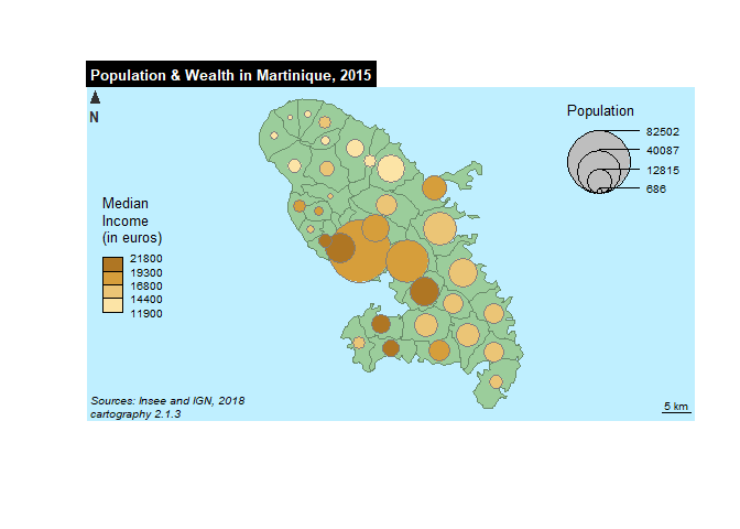
The cheatsheet for the cartography package should be highlighted here as well!
1.3 Interactive maps with map view
Sometimes there is a need to navigate around a map or visually inspect items from it. Here the mapview package can help. It renders any spatial object on top of a leaflet map. This functionality requires internet access and works with most spatial objects (sp, sf, raster, etc…)!
library(mapview)## Warning: package 'mapview' was built under R version 4.0.3library(raster)## Loading required package: sp##
## Attaching package: 'raster'## The following object is masked from 'package:dplyr':
##
## select# Get the forest raster
forest <- raster('ht_004_clipped.tif',1)
# Divide by 1000 to get fractions
forest <- forest / 1000
# Let us render the forest layer
# Some warnings might pop due to the number of pixels exceeding the amount that can be rendered efficiently. However mapview will automatically suggest lower numbers for rendering
# Topo colors here
pal = mapviewPalette("mapviewTopoColors")
mapview(forest, col.regions = rev( pal(100) ),
na.color = NA,
layer.name = 'Forest fraction'
)## Warning in rasterCheckSize(x, maxpixels = maxpixels): maximum number of pixels for Raster* viewing is 5e+05 ;
## the supplied Raster* has 521909
## ... decreasing Raster* resolution to 5e+05 pixels
## to view full resolution set 'maxpixels = 521909 '## Warning in showSRID(uprojargs, format = "PROJ", multiline = "NO"): Discarded
## ellps WGS 84 in CRS definition: +proj=merc +a=6378137 +b=6378137 +lat_ts=0
## +lon_0=0 +x_0=0 +y_0=0 +k=1 +units=m +nadgrids=@null +wktext +no_defs## Warning in showSRID(uprojargs, format = "PROJ", multiline = "NO"): Discarded
## datum WGS_1984 in CRS definition## Warning in showSRID(uprojargs, format = "PROJ", multiline = "NO"): Discarded
## ellps WGS 84 in CRS definition: +proj=merc +a=6378137 +b=6378137 +lat_ts=0
## +lon_0=0 +x_0=0 +y_0=0 +k=1 +units=m +nadgrids=@null +wktext +no_defs## Warning in showSRID(uprojargs, format = "PROJ", multiline = "NO"): Discarded
## datum WGS_1984 in CRS definitionNote that each object (point or raster grid cell) on the map viewer can be queried and clicked. Try to navigate around a bit.
A lot more examples and visualization tricks can be found on the mapview homepage.
Can you render the Laxenburg park?
# Add the laxenburg Park
laxpol <- st_read('Laxenburg.gpkg')
mapview(laxpol)